MultiPeriod Portfolio Optimization: Beyond One-Step-Ahead Thinking

Some theory and practice

I must admit, the AI did a good job helping me write all this below but the crucial points and code is mine.

Introduction

Portfolio optimization has been a cornerstone of quantitative finance since Harry Markowitz introduced Modern Portfolio Theory in the 1950s. The traditional approach optimizes portfolios for a single future period, making allocation decisions based on expected returns and risks for that period alone.

But markets evolve continuously, and optimal decisions today depend on what might happen not just tomorrow, but in the days, weeks, and months that follow. This is where multiperiod optimization enters the picture.

In this article, I'll dive into the implementation and execution of a multiperiod optimization framework for portfolio management 1) building on the framework developed by Boyd et al. (2017), 2) using the latest cvxportfolio library (version 1.0+). I'll explore not just the theory, but the nuts and bolts of how to properly build such a system.

---

What is Multiperiod Optimization?

MPO solves a sequential decision-making problem over a finite horizon T. Unlike myopic single-period optimizers, it recognizes three critical realities:

1. Path-dependent costs: Trading at time t alters available capital at t+1

2. Convex market impact: Large trades incur superlinear costs

3. Time-varying opportunities: Expected returns μt​ and risks Σ^t​ evolve dynamically

MPO problem maximizes utility over a receding horizon H, balancing returns, risk, and transaction costs. Assuming a portfolio of N assets, the optimization at time t solves:

\({\{\mathbf{w}_{t+1}, \ldots, \mathbf{w}_{t+H}\}} \sum_{\tau=t+1}^{t+H} \left( \hat{\mathbf{r}}_{\tau}^{\mathsf{T}} \mathbf{w}_{\tau} - \gamma^{\text{risk}} \mathbf{w}_{\tau}^{\mathsf{T}} \hat{\Sigma}_{\tau} \mathbf{w}_{\tau} - \gamma^{\text{trade}} \sum_{i=1}^N T\!C(\Delta w_{i,\tau}) \right)\)

subject to:

\(\quad \mathbf{1}^{\mathsf{T}} \mathbf{w}_{\tau} = 1, \quad \mathbf{w}_{\tau} \geq 0.01 \quad \forall \tau \in \{t+1, \ldots, t+H\}\)

where:

1. Decision Variables:

   • wτ​: Portfolio weights at time τ (N×1 vector); here constrained to be at least 1% per each asset and long-only.

   • Δwi,τ​ = wi,τ​−wi,τ−1​: Change in weight for asset i.

2. Return Estimates:

   • r^τ​: Estimated returns (N×1 vector), coming from a model of choice.

3. Risk Penalty:

   • Σ^τ​: Rolling covariance matrix (N×N)

   • γrisk: Risk-aversion parameter (can be tuned via hyperparameter optimization; the higher the more risk averse).

4. Transaction Costs:

   \(T\!C(\Delta w_{i,\tau}) = \frac{b}{2} P_{i,\tau-1} |\Delta w_{i,\tau}| + \text{EMA}_{\sigma_{i,\tau-1}} \frac{|\Delta w_{i,\tau}|^{1.5}}{\left(\frac{\text{EMA}_{v_{i,\tau-1}}}{V_{\tau-1}}\right)^{0.5}}\)

   1. b: bid/ask spread

   2. EMAσ​, EMAv​: Volatility and volume estimates

   3. Vτ​: Total portfolio trading volume.

5. Hyperparameters:

   • γtrade: Penalty for turnover (can be tuned via hyperparameter optimization; the higher, the lower portfolio turnover).

   • H: Optimization horizon.

The framework, more or less works like this (for H = 3):

---

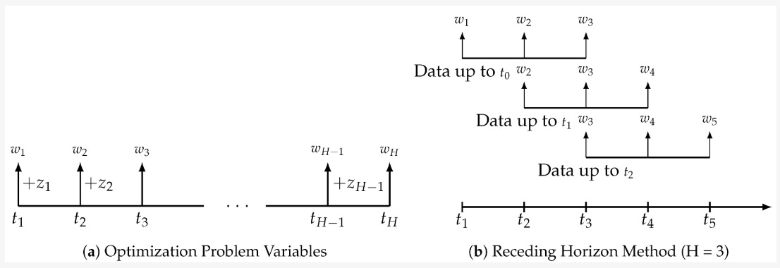
Data Preparation

Before diving into the optimization itself, we need to prepare several key inputs:

Asset Returns

Given the optimization formula above, we need both historical returns (for risk modeling) and expected future returns (for optimization). In this implementation this is actually up to you but best to just use a linear regression for starters (or whatever you find interesting in this article).

Transaction Costs

For the transaction costs component, it’s best to initially follow the paper’s assumptions:

1. A linear component (half-spread) → 20 bps

2. A non-linear component:

   1. Expected asset volatility (sigma) → exponential moving std over 10 days

   2. Expected asset volume → exponential moving average over 10 days

Risk Estimates

For risk components, the Σ^t could basically be a rolling full covariance matrix with a lookback period of 504 days (again, the paper’s number).

---

Implementation Process

Let's now move on to the key steps of implementing multiperiod optimization with the cvxportfolio package:

Data Loading and Processing

The first step is to load and process data for different asset classes. You can use a cross-asset portfolio or a single one; it’s up to you but probably it’s best to start with a unified portfolio with, for instance, equities or cryptocurrencies.

For each asset group, you must have these prepared:

• Actual returns (for backtesting)

• Expected returns (for optimization)

• Actual sigmas and volumes (for simulating transaction costs)

• Estimated sigmas and volumes (for modeling expected transaction costs)

The data processing involves:

• Aligning all datasets to the same index (to make sure there is no leak)

• Handling missing values with forward-filling (the package does not like NaNs)

• Applying appropriate time shifts to ensure no lookahead bias (yeah)

Creating a Custom Returns Forecast

A key component of multiperiod optimization is the returns forecast. In the package, this is handled by creating a custom forecast object:

class CustomReturnsForecast(cp.ReturnsForecast):
    def __init__(self, est_returns_df, horizon):
        super().__init__()
        self.est_returns_df = est_returns_df
        self.horizon = horizon
        
    def values_in_time(self, t, tau=None):
        """Return forecasted values at time t for time tau."""
        if tau is None or tau == t:
            return self.est_returns_df.loc[t]
        
        # Find the index position of t
        try:
            idx = self.est_returns_df.index.get_loc(t)
            future_idx = idx + (tau - t).days
            
            if future_idx < len(self.est_returns_df):
                future_date = self.est_returns_df.index[future_idx]
                return self.est_returns_df.loc[future_date]
        except (KeyError, TypeError):
            pass
        
        # Default fallback, use t's forecast
        return self.est_returns_df.loc[t]

This class implements the values_in_time method, which provides return forecasts for different time points in the future. Again, the method carefully handles time indexing to prevent lookahead bias.

Building the Optimization Models

With the data prepared, we can build several models required for optimization:

# Risk model based on historical returns
risk_model = cp.FullCovariance(returns_for_sigma_df.shift().dropna(), lookback=RISK_LOOKBACK_DAYS)

# Transaction cost model based on expected volatility and volume
transaction_cost = cp.TransactionCost(
    half_spread=HALF_SPREAD, 
    nonlin_coeff=NONLIN_COEFF, 
    sigma=est_sigmas_df.shift(),
    volume=est_volumes_df.shift()
)

# Holding cost model (optional)
holding_cost = cp.HoldingCost(borrow_costs=BORROW_COSTS)

Where RISK_LOOKBACK_DAYS is 504, HALF_SPREAD is 20bps, NONLIN_COEFF is 1.0 (so no effect on estimates), and BORROW_COSTS are close to 0, since holding_cost is actually a component that applies only to short positions, while we are only interested in short positions.

In the latest cvxportfolio version, the models are combined using arithmetic operations to create a comprehensive objective function:

combined_objective = returns_forecast - (
    gamma_risk_pareto * risk_model +
    gamma_tcosts_pareto * transaction_cost +
    gamma_holdings_pareto * holding_cost (optional)
)

Where:

• gamma_risks_pareto: Weight on risk minimization (γrisk)

• gamma_tcosts_pareto: Weight on transaction cost minimization (γtrade)

• gamma_holdings_pareto: Weight on holding cost minimization (optional)

This expression balances expected returns against various costs: risk (volatility), transaction costs, and optional holding costs. The gamma parameters control the relative sensitivity of our portfolio to each component.

Constructing the Multi-Period Policy

The policy is created using the MultiPeriodOptimization class, which takes the combined objective function, constraints, and planning horizon:

policy = cp.MultiPeriodOptimization(
    objective=combined_objective,
    constraints=[cp.LongOnly(), cp.MinWeights(0.01)],
    planning_horizon=HORIZON
)

Here, obviously, the planning_horizon parameter specifies how many periods to look ahead when making trading decisions. The horizon (H) is of course a critical parameter; however, to choose it we must remember the following:

• The longer the horizon, the potentially better protected and adapted portfolio. But…

• …the longer the horizon, the more computationally expensive the optimization and…

• …the more difficult for the estimates to work accurately.

You can choose between 2-5 for starters; if monthly, then 3 is fine, while weekly or daily maybe 5.

Hyperparameter Optimization

As mentioned previously, MPO involves balancing different objectives, controlled by hyperparameters γrisk and γtrade. The paper checks several; however, we can use Optuna to find the optimal values, although using the proposed parameters as starting and ending numbers.

def objective(trial):
    params = {
        "gamma_risks_pareto": trial.suggest_float("gamma_risks_pareto", 0.01, 1000.0),
        "gamma_tcosts_pareto": trial.suggest_float("gamma_tcosts_pareto", 0.0001, 25.0),
    }

    # Create combined objective with the trial parameters
    combined_objective = returns_forecast - (
        params["gamma_risks_pareto"] * risk_model +
        params["gamma_tcosts_pareto"] * transaction_cost +
    )
    
    # Create policy and run backtest
    policy = cp.MultiPeriodOptimization(
            objective=combined_objective,
            constraints=constraints,
            planning_horizon=HORIZON,
            # The new API handles trading times internally
        )

    simulation = simulator.backtest(
                policy,
                initial_portfolio=init_portfolio, 
                start_time=start_train, 
                end_time=end_train
        )
    
    # Return Sharpe ratio as the optimization metric
    return simulation.sharpe_ratio

Where init_portfolio is just a starting cash for the backtested assets, e.g.,:

init_portfolio = pd.Series(index=returns_df.columns, data=25000.0)

while end_t is the last timestamp of the training set.

Final Simulation

Once you’ve found the optimal hyperparameters, you can run a final simulation on out-of-sample data to evaluate the performance of your multiperiod optimization strategy:

# Create policy with best parameters
combined_objective = returns_forecast - (
    gamma_risk_pareto * risk_model +
    gamma_tcosts_pareto * transaction_cost +
)

final_policy = cp.MultiPeriodOptimization(
    objective=combined_objective,
    constraints=constraints,
    planning_horizon=HORIZON
)

# Run backtest comparing against a Hold policy
final_simulation = simulator.run_multiple_backtest(
    policies=[cp.Hold(), final_policy],
    initial_portfolio=init_portfolio,
    start_time=start_test,
    end_time=end_test
)

Where between end_train and start_test there is a sufficient gap so that estimates are properly purged. In addition, here we compare my optimized policy against a simple "hold" policy to see the added value of multiperiod optimization.

---

Results

I can show you the results I got back in my PhD; however, here a lot of work was done by my model that predicted returns plus the trick with lagged Kalman Filter I did to potentially correct wrong estimates

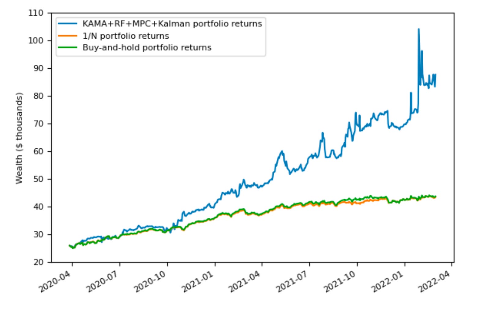
The out of sample period had a bit over 2 years and stopped in March 2022 where I finished my experiment. As you can see, the portfolio is pretty volatile but that’s because my optimal parameters were:

• γrisk = 0.13

• γtrade = 4.7

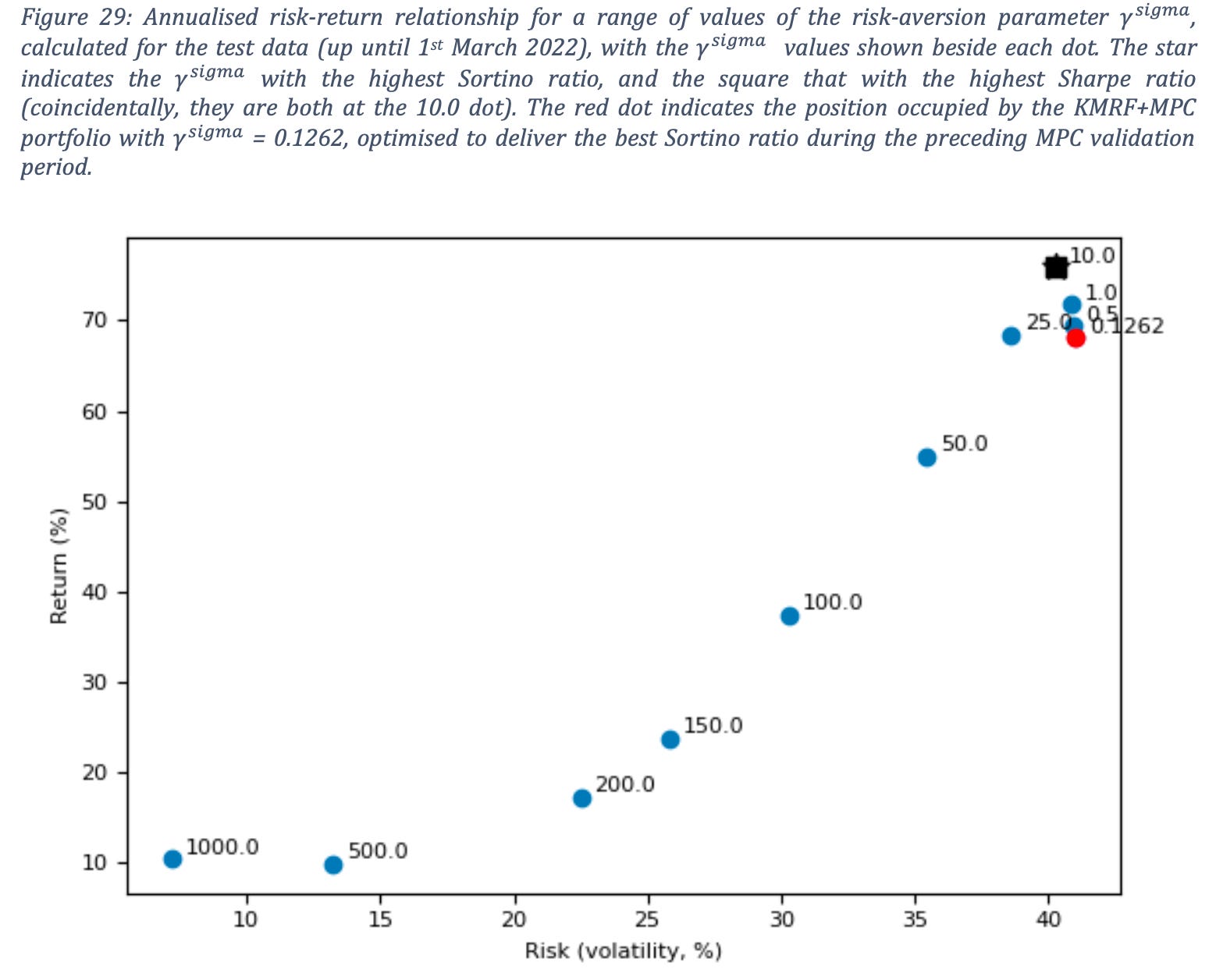
The values mean that the portfolio is far away from risk aversion but makes sure there is no high turnover due to increased costs. In other words, it prefers keeping highly vol assets for a longer period over trading them. When I set γrisk to be way higher, I got:

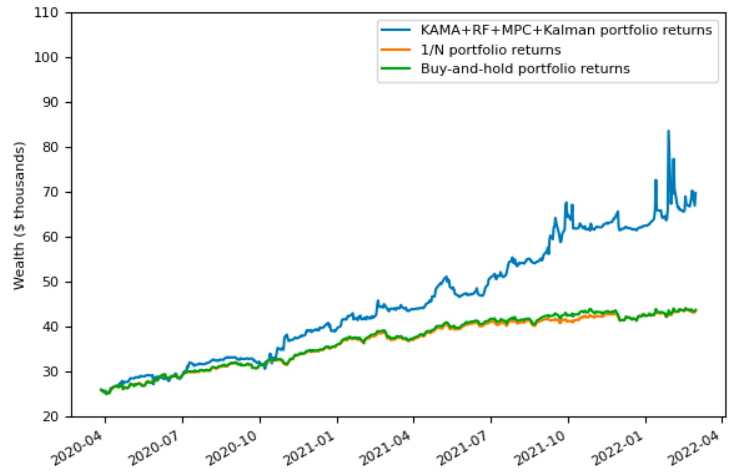
Still volatile but not that much. For various γrisk (sigma) values and their effect on risk/return profile, you can adhere to this chart:

---

Discussion

Benefits of Multiperiod Optimization

MPO generally offers several advantages over traditional single-period approaches:

1. Transaction Cost Awareness: By considering multiple future periods, the optimizer can spread trades over time to minimize transaction costs. This is particularly important for large portfolios or less liquid markets.

2. Forward-Looking Risk Management: The approach considers how risk evolves over time, not just the immediate risk profile.

3. Adaptivity to Changing Market Conditions: The optimizer can plan for expected changes in market conditions, adjusting the portfolio gradually rather than reactively.

Challenges and Limitations

Despite its advantages, multiperiod optimization comes with challenges; apart from the horizon and forecast limitations I mentioned, there also is:

1. Hyperparameter Sensitivity: Finding the right balance between risk, return, and cost objectives can be challenging and may require frequent recalibration.

2. Implementation Complexity: As shown in the code, implementing a robust multiperiod optimization framework requires careful attention to data processing, model building, and simulation.

---

AI Conclusion

Multiperiod optimization represents a significant advancement in portfolio management, moving beyond the limitations of traditional single-period approaches. By considering a sequence of future periods simultaneously, it allows for more strategic decision-making that accounts for transaction costs, time-varying investment opportunities, and the impact of current decisions on future flexibility.

The implementation above demonstrates the practical steps involved in building a multiperiod optimization framework using cvxportfolio: from data preparation and model building to hyperparameter optimization and performance evaluation. While the approach requires more sophisticated modeling and computational resources, the potential improvements in risk-adjusted returns make it a valuable tool for quantitative portfolio managers.

If you are interested, you can check out a bunch of examples in the official repo.